Thesis template manual - Advanced functionality

Display all bibliography
Bibliography style
Two-side document
Extra packages
1. Local installation
R and LaTeX
Tools for benchmarking

Display all bibliography

The final version of the paper should not include a list of literature sources that are not referenced at all in the paper. However, at the writing stage of the work, it may be useful to show the entire list, for example, to facilitate the work of the supervisor. The following document lists all the literature:

\documentclass[language=english]{utuftthesis}

\addbibresource{Bibliografia.bib}

\begin{document}

\publab{Labran nimi}
\publaben{Laboratory Name}
\pubtype{msc}
\title{Name of Thesis}
\author{My Name}

\maketitle

% command for controlling the visibility of
% bibliography entries
\nocite{*}

\printbibliography

\end{document}

You could even create a distinct root document for displaying this list. Using the same document class (utuftthesis.cls) is recommended because that way the bibliography list will have the same style for formatting.

Bibliography style

The utuftthesis.cls template defaults to using the biblatex package (ieee style) and the Biber engine to generate bibliographies and citations.

The following resources may help with the biblatex configuration:

To change the bibliography style, just redefine the style in the document header:

\documentclass[language=finnish,bibstyle=ieee]{utuftthesis}

...

\end{document}

Preview of the default (ieee) bibliography style:

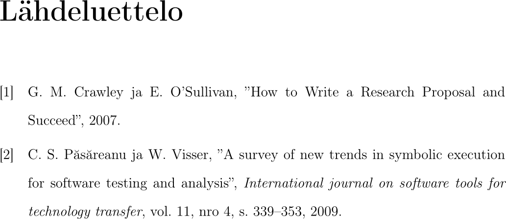
Citations:

For example, to use the alphabetic style, replace the code with:

\documentclass[language=finnish,bibstyle=alphabetic]{utuftthesis}

...

\end{document}

Preview of the alphabetic bibliography style:

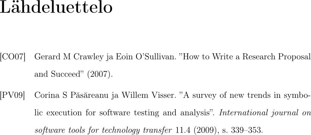
Citations:

For more advanced configuration, the relevant biblatex configuration entries can be found in the utuftthesis.cls file:

%% bibliography, new engine
\ifdefstring{\utuftthesis@biburlbreak}{ragged}{
  \RequirePackage[style=\utuftthesis@bibstyle,backend=biber,block=ragged]{biblatex}
}
{
  \RequirePackage[style=\utuftthesis@bibstyle,backend=biber]{biblatex} 
}

Two-side document

Preliminary support for two-side documents was added in 2023/08/02. The two-side document reverses the left and right margins for even pages. To enable this mode, add the sides=twoside key-val pair to the document class configuration line:

\documentclass[language=finnish,sides=twoside]{utuftthesis}

Please note that the two-side document still has issues switching between even and odd page formatting when switching between sections (e.g. TOC, main document, bibliography, appendices). You can manually add empty pages with the \newpage command to the end of each section when needed.

This suggested solution can also be used to automatically add the necessary empty pages.

Extra packages

The LaTeX ecosystem provides a variety of extra packages that are not available in our Docker image. Should a required package be missing, see http://www.ctan.org/. Consultation of the manuals of these packages is strongly encouraged.

The TexLive distribution used by the thesis projects provides a package manager of its own. The recommended approach for installing these packages is to either use a local TeX installation or to create a custom Docker image, then to configure the CI/CD script to use this new image.

❗ Installing packages in the GitLab CI/CD script is not recommended as the script is run after each commit. This can generates extra traffic to CTAN servers and the repositories may even block access to fight the bandwidth costs. ❗

Local installation

Assuming a local LaTeX distribution has been set up, the tlmgr command can be used to install more packages:

$ tlmgr update --self
$ tlmgr install MYPACKAGE1 MYPACKAGE2

If the document will be recompiled multiple times and/or one needs to experiment with new packages, the local installation is probably the most efficient approach.

R and LaTeX

Knitr can be used for embedding R code in TeX files. Knitr supports caching of the generated figures to improve performance. A previously installed R distribution is required to use Knitr.

One can begin with this simple example.Rnw:

\documentclass{article}
\usepackage[utf8]{inputenc}
\usepackage[english]{babel}
 
\begin{document}
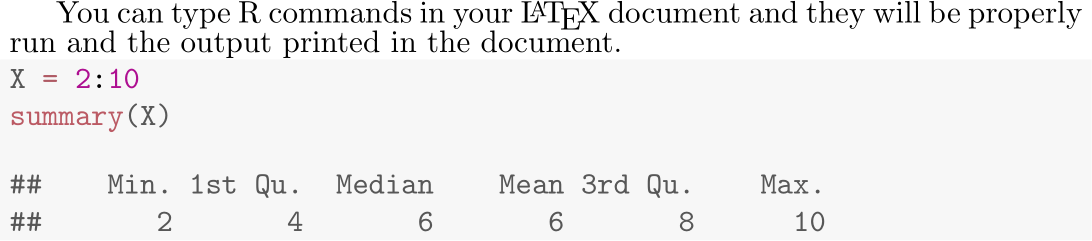
You can type R commands in your \LaTeX{} document and they will be 
properly run and the output printed in the document.
 
<<>>=
X = 2:10
summary(X)
@

\end{document}

First, process the embedded R code with R & Knitr:

$ Rscript -e "library(knitr); knit('example.Rnw')"

The script generates all the figures, and produces a normal .tex file with the textual content pre-rendered inline:

...
\begin{document}
You can type R commands in your \LaTeX{} document and they will be 
properly run and the output printed in the document.
 
\begin{knitrout}
\definecolor{shadecolor}{rgb}{0.969, 0.969, 0.969}\color{fgcolor}\begin{kframe}
\begin{alltt}
\hlstd{X} \hlkwb{=} \hlnum{2}\hlopt{:}\hlnum{10}
\hlkwd{summary}\hlstd{(X)}
\end{alltt}
\begin{verbatim}
##    Min. 1st Qu.  Median    Mean 3rd Qu.    Max. 
##       2       4       6       6       8      10
\end{verbatim}
\end{kframe}
\end{knitrout}

\end{document}

The generated file can be compiled with LaTeX:

$ latexmk -pdf -shell-escape example.tex